# Function to process exams
process_exam <- function(exam_path, question_id) {

  exam <- read.csv(file.path("~", exam_path))

  exam_q1 <- as.data.table(exam)[Question.ID == question_id ,c("Username","Answer")]

  exam_q1$Answer <- gsub("<.*?>", "", exam_q1$Answer)

  exam_q1_corpus <- corpus(exam_q1, docid_field = "Username", text_field  ="Answer")

  exam_q1_dfm <- dfm(exam_q1_corpus %>% tokens(), tolower= TRUE, remove_padding = TRUE)

  tstat_hist <- textstat_simil(exam_q1_dfm, method = "cosine", margin = "documents")

  tstat_hist_vector <- as.vector(tstat_hist)

  tstat1 <- textstat_simil(exam_q1_dfm, method = "cosine", margin = "documents", min_simil = 0.9)

  potential_cheater <- as.data.frame(as.table(as.matrix(tstat1)))
  potential_cheater <- na.omit(potential_cheater)

  names(potential_cheater) <- c("id1", "id2", "cosine")

  potential_cheater <- potential_cheater %>%
    mutate(cheaters = ifelse((cosine!=1 & (id1!=id2)),1,0)) %>%
    filter(cheaters ==1)

  potential_cheater <- potential_cheater[which(!duplicated(potential_cheater$cosine)),]

  #list(tstat_hist_vector = tstat_hist_vector, potential_cheater = potential_cheater)

    # Create a list to keep track of the source file and question ID
    result <- list(
    file = exam_path,
    question_id = question_id,
    data = tstat_hist_vector,
    potential_cheater = potential_cheater)
}

path_files <- list.files(pattern =".csv", path = "~/Dropbox/welda_website/cheating/csv")

online_files   <- path_files[1:3]
offline_files  <- path_files[4]

online_questions <- c(1, 2)
offline_questions <- c(18, 19)Data Science in Action: Detecting Cheaters with Cosine Similarity
Introduction
In this blog, we will endeavor to devise a code that identifies potential cheaters using cosine similarities of answers. A friend, who happens to be an educator, approached me seeking a quick and efficient way to detect potential cheaters and review their submissions. However, due to the ambiguous nature of mathematical expressions in the answers, the features provided by Blackboard couldn’t be of much assistance. Therefore, I formulated an R code to assist my friend in pinpointing students who might be cheating. The students’ IDs have been encrypted by my friend and hence, carry no significance to me. The following steps outline the procedure to detect potential cheaters:
Setting Up the libraries
Setting Up the libraries: Here, necessary libraries for the analysis are loaded. These include libraries for data manipulation (dplyr, data.table, tidyr), text analysis (quanteda, quanteda.textstats), visualization (ggplot2, kableExtra, igraph, networkD3, network, tidygraph, ggraph), and the knitr library for neat output formatting.
The process_exam function: This function performs the main cheating detection analysis. It takes an exam file and a question ID as inputs. It reads the exam file, selects the answers for the specified question, removes HTML tags, and constructs a document-feature matrix. Cosine similarities between answers are computed and potential cheaters are identified as those pairs of answers with cosine similarity above 0.9 (excluding identical answers).
Online class and Offline class: These sections call the process_exam function for each exam file (online and offline) and each question. The result is a list of results for each file and question.
Online class
online_files <- paste0("Dropbox/welda_website/cheating/csv/", online_files)

# Process online exams
online_results <- lapply(online_files, function(file) {
  # Loop over the range of online question IDs
  lapply(1:2, function(question_id) {
    process_exam(file, question_id = question_id)
  })
})
Offline class
offline_files <- paste0("Dropbox/welda_website/cheating/csv/", offline_files)

# Process offline exams
offline_results <- lapply(offline_files, function(file) {
  # Loop over the range of offline question IDs
  lapply(18:19, function(question_id) {
    process_exam(file, question_id = question_id)
  })
})
Density of the cosine similarities
Density of the cosine similarities: These sections create density plots of the cosine similarities between student answers. These plots provide a visual representation of the distribution of answer similarity, with a vertical line at 0.9 indicating the threshold for detecting potential cheating.
# Combine the tstat vectors for each question in the online exams
online_tstats_q1 <- lapply(online_results, function(file_result) {
  file_result[[1]]$data
})

online_tstats_q2 <- lapply(online_results, function(file_result) {
  file_result[[2]]$data
})

# Combine the tstat vectors for each question in the offline exams
offline_tstats_q1 <- lapply(offline_results, function(file_result) {
  file_result[[1]]$data
})

offline_tstats_q2 <- lapply(offline_results, function(file_result) {
  file_result[[2]]$data
})


# Create a data frame with each list as a separate row
tstat_data_q1 <- data.frame(
  tstats = c(unlist(online_tstats_q1[[1]]), unlist(online_tstats_q1[[2]]), unlist(online_tstats_q1[[3]]), unlist(offline_tstats_q1)),
  section = rep(c('online_1', 'online_2', 'online_3', 'offline'), times = c(length(unlist(online_tstats_q1[[1]])),
                                                                            length(unlist(online_tstats_q1[[2]])),
                                                                            length(unlist(online_tstats_q1[[3]])),
                                                                            length(unlist(offline_tstats_q1))))
)


tstat_data_q2 <- data.frame(
  tstats = c(unlist(online_tstats_q2[[1]]), unlist(online_tstats_q2[[2]]), unlist(online_tstats_q2[[3]]), unlist(offline_tstats_q1)),
  section = rep(c('online_1', 'online_2', 'online_3', 'offline'), times = c(length(unlist(online_tstats_q2[[1]])),
                                                                            length(unlist(online_tstats_q2[[2]])),
                                                                            length(unlist(online_tstats_q2[[3]])),
                                                                            length(unlist(offline_tstats_q1))))
)

library(ggplot2)
library(tidyr)

# Plot the densities
ggplot(tstat_data_q1, aes(x = tstats, fill = section)) +
  geom_density(alpha = 0.5) +
  geom_vline(xintercept = 0.9, linetype = "dashed", color = "red", size = 1) +
  labs(title = "Density of cosine similarity between questions from different exams - question 1",
       x = "Cosine Similarity",
       y = "Density") +
  scale_fill_manual(values = c("online_1" = "#FF6347", "online_2" = "#ADD8E6", "online_3" = "#90EE90", "offline" = "#800080")) +
  theme_minimal() +
  theme(legend.title = element_blank()) +
  annotate("text", x = 0.9, y = 5, label = "Potential Cheaters", hjust = 1.2, color = "red")
When examining the distribution of cosine similarities, an intriguing observation arises: the offline class appears to skew more to the left in comparison to the online class, which exhibits a higher frequency for greater values of cosine similarities. This suggests that students in the online class are likely to cheat more frequently than those in the offline class. My friend noted that students tend to be more engaged in the offline class compared to the online one, so this outcome is not entirely surprising - in fact, it aligns with our expectations.
# Plot the densities
ggplot(tstat_data_q2, aes(x = tstats, fill = section)) +
  geom_density(alpha = 0.5) +
  geom_vline(xintercept = 0.9, linetype = "dashed", color = "red", size = 1) +
  labs(title = "Density of cosine similarity between questions from different exams - question 2",
       x = "Cosine Similarity",
       y = "Density") +
  scale_fill_manual(values = c("online_1" = "#FF6347", "online_2" = "#ADD8E6", "online_3" = "#90EE90", "offline" = "#800080")) +
  theme_minimal() +
  theme(legend.title = element_blank()) +
  annotate("text", x = 0.9, y = 5, label = "Potential Cheaters", hjust = 1.2, color = "red")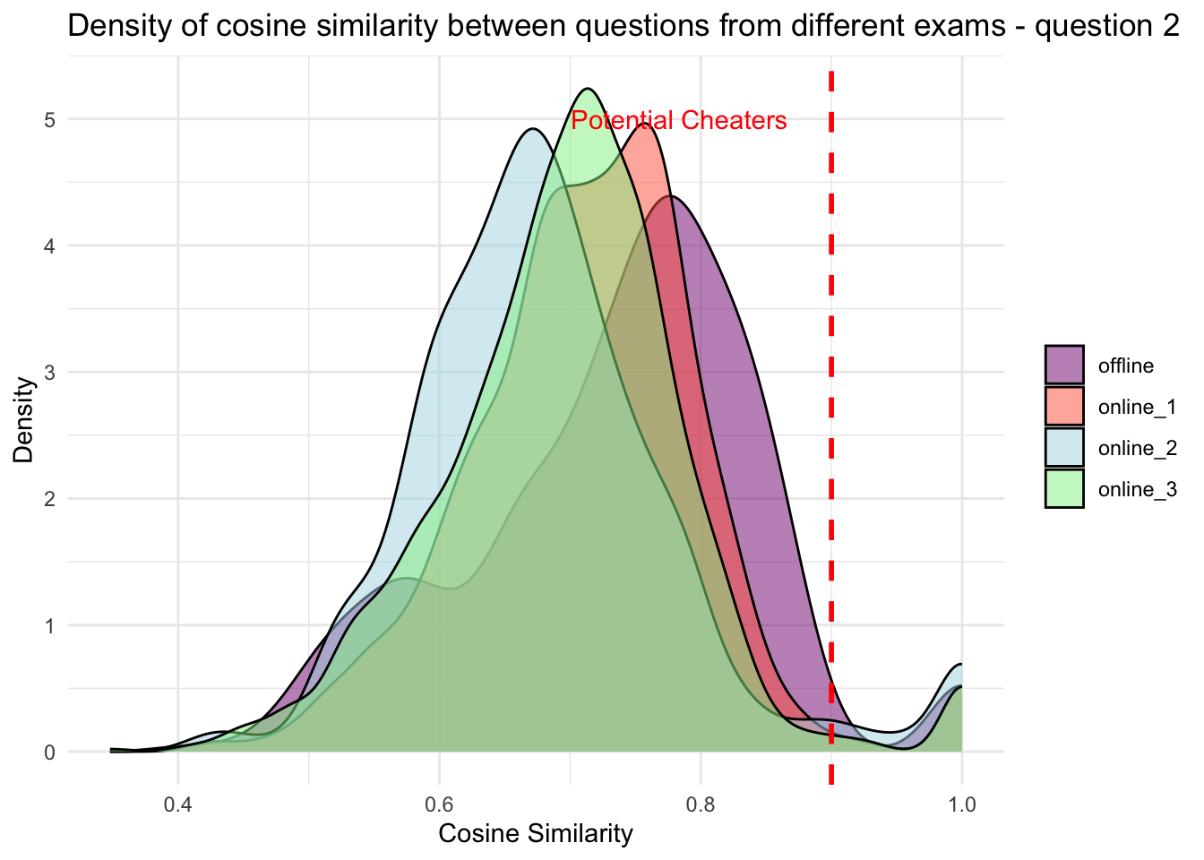
Investigating the possible network of Cheaters in one of online sections
Investigating the possible network of Cheaters in one of online sections: This section visualizes potential cheaters as a network graph, where nodes represent students and edges represent potential cheating incidents. This visual representation can be useful for understanding the relationships between potential cheaters.
# Combine the cheaters vectors for each question in the online exams
online_cheaters <- lapply(online_results, function(file_result) {
  rbind(file_result[[1]]$potential_cheater,
        file_result[[2]]$potential_cheater)

})


# Combine the cheaters vectors for each question in the offline exams

offline_cheaters <- lapply(offline_results, function(file_result) {
   rbind(file_result[[1]]$potential_cheater,
         file_result[[2]]$potential_cheater)

})

# cheaters for section one
potential_cheater  <- online_cheaters[[1]]
potential_cheater <- potential_cheater %>% arrange(desc(cosine))
knitr::kable(head(potential_cheater), booktabs = T) %>%
kable_styling(position = "center",latex_options = "HOLD_position")| id1 | id2 | cosine | cheaters | |
|---|---|---|---|---|
| 10 | XDQ114120107 | BDY118120115 | 0.9426680 | 1 |
| 8 | YDS115120111 | TDQ110120107 | 0.9404906 | 1 |
| 14 | YDS115120110 | XDQ114120107 | 0.9400602 | 1 |
| 61 | YDH115120099 | GDI097120099 | 0.9389956 | 1 |
| 12 | ITT099110110 | BDY118120115 | 0.9311809 | 1 |
| 29 | RDA108120117 | HDJ098120100 | 0.9302268 | 1 |
# Create a data frame with potential cheaters
data <- data.frame(
  Source = potential_cheater$id1,
  Target = potential_cheater$id2
)

# Plot the network graph
p <- simpleNetwork(data, height = "150px", width = "100px",
                   Source = 1,         # Column number of source
                   Target = 2,         # Column number of target
                   linkDistance = 10,  # Distance between nodes
                   charge = -900,      # Strength of node repulsion
                   fontSize = 24,      # Size of node names
                   fontFamily = "serif",  # Font of node names
                   linkColour = "#666",   # Colour of edges
                   nodeColour = "#609960",  # Colour of nodes
                   opacity = 0.9,      # Opacity of nodes
                   zoom = TRUE         # Enable zoom
)

p
Note
You can interact with the network graph above by zooming in and out for more detailed views.
Upon studying the network graph of potential cheaters, we observe some intriguing patterns. There’s a clear network of students who have strikingly similar answers, indicative of potential cheating.
What’s particularly interesting is how this network might be able to tell us where the cheating originated. By examining the centrality of this network, we can identify which students are most connected to others - these are students whose answers bear similarity to many others’. In network theory, such nodes are often considered influential within the network, because they interact with a large number of other nodes.
However, it’s crucial to approach this with caution. While a student being at the ‘center’ of this network could imply that they are the source of the copied answers, there could be other explanations as well. It’s also possible that this student’s work was shared without their consent. As such, while this method can identify suspicious patterns, further investigation will be required to definitively determine any cases of academic dishonesty. Nonetheless, by scrutinizing such networks, we have a powerful tool to identify potential instances of cheating, and further probe into the specifics.